visualize

Generic spatial visualization: render any ee.Image, export PNGs, GIFs, and timestrips.

Visualization Parameters

A simple wrapper for GEE visualization parameters.

---

source

VisParams

def VisParams(
    min:Optional=None, max:Optional=None, palette:Optional=None, bands:Optional=None, gamma:Optional=None
)->None:

Visualization parameters for rendering layers.

Examples: # For single-band continuous data (NDVI, temperature) VisParams(min=-0.2, max=0.8, palette=[‘red’, ‘yellow’, ‘green’])

# For RGB composites
VisParams(min=0, max=0.3, bands=['B4', 'B3', 'B2'], gamma=1.4)

# For categorical data
VisParams(min=0, max=7, palette=['#111', '#ccc', '#0f0', ...])

Core Rendering Functions

These are the building blocks - they work with any ee.Image.

---

source

render_thumbnail

def render_thumbnail(
    image:Image, region:Geometry, vis_params:dict, dimensions:int=512, format:str='png'
)->bytes:

Render an ee.Image to thumbnail bytes.

Args: image: The image to render region: Region to render vis_params: Visualization parameters dict dimensions: Max dimension in pixels format: Image format (‘png’ or ‘jpg’)

Returns: Image bytes

---

source

add_label

def add_label(
    img:Image, label:str, position:Literal='bottom-left', font_size:int=16, text_color:str='white',
    bg_color:str='black', padding:int=5
)->Image:

Add a text label to an image.

Generic Image Rendering

The core render_image function works with any ee.Image.

---

source

render_image

def render_image(
    image:Image, region:Geometry, vis_params:Union, dimensions:int=512, boundary:Optional=None,
    boundary_color:str='#FFFFFF', boundary_width:int=2, label:Optional=None, label_position:str='bottom-left'
)->Image:

Render any ee.Image to a PIL Image.

This is the core generic rendering function. It works with any ee.Image from any source (Sentinel, MODIS, Landsat, custom computations, etc.).

Args: image: Any ee.Image to visualize region: Region to render (usually site.geometry.buffer(n).bounds()) vis_params: Visualization parameters (VisParams or dict) dimensions: Image size in pixels boundary: Optional geometry to overlay as boundary line boundary_color: Color for boundary line boundary_width: Width of boundary line label: Optional text label label_position: Position for label

Returns: PIL Image

Example: # Get any ee.Image from any source image = ee.Image(‘USGS/SRTMGL1_003’) # elevation

# Render it
pil_img = render_image(
    image=image,
    region=site.geometry.buffer(1000).bounds(),
    vis_params={'min': 0, 'max': 3000, 'palette': ['green', 'yellow', 'brown']},
    boundary=site.geometry,
    label='Elevation'
)

Layer-Based Rendering

Convenience functions for rendering CategoricalLayer and ContinuousLayer objects.

---

source

get_image_for_layer

def get_image_for_layer(
    layer:Union, geometry:Geometry, year:Optional=None, date_range:Optional=None, reducer:str='median'
)->Image:

Get an ee.Image from a CategoricalLayer or ContinuousLayer.

---

source

get_vis_params_from_layer

def get_vis_params_from_layer(
    layer:CategoricalLayer
)->dict:

Extract visualization params from a CategoricalLayer’s palette.

---

source

render_site_layer

def render_site_layer(
    site:Site, layer:Union, year:Optional=None, date_range:Optional=None, vis_params:Union=None, buffer_m:float=500,
    dimensions:int=512, show_boundary:bool=True, boundary_color:str='#FFFFFF', boundary_width:int=2,
    label:Optional=None, label_position:str='bottom-left'
)->Image:

Render a CategoricalLayer or ContinuousLayer for a site.

This is a convenience wrapper around render_image() for Layer objects.

Generic Export Functions

These work with any rendering function via a “frame generator” pattern.

---

source

export_frames_as_strip

def export_frames_as_strip(
    frames:list, output_path:Union, orientation:Literal='horizontal', spacing:int=2, background_color:str='#000000'
)->Path:

Export a list of PIL Images as a strip (side by side).

Args: frames: List of PIL Images (should be same size) output_path: Output file path orientation: ‘horizontal’ or ‘vertical’ spacing: Pixels between tiles background_color: Background color

Returns: Path to saved file

---

source

export_frames_as_gif

def export_frames_as_gif(
    frames:list, output_path:Union, duration_ms:int=500, loop:bool=True
)->Path:

Export a list of PIL Images as animated GIF.

Args: frames: List of PIL Images output_path: Output file path duration_ms: Frame duration in milliseconds loop: Whether to loop

Returns: Path to saved file

High-Level Export Functions

Convenient wrappers for common use cases with Layer objects.

---

source

export_layer_timestrip

def export_layer_timestrip(
    site:Site, layer:Union, output_path:Union, years:list, vis_params:Union=None, buffer_m:float=500,
    tile_size:int=256, show_boundary:bool=True, boundary_color:str='#FFFFFF', add_labels:bool=True,
    orientation:Literal='horizontal', spacing:int=2
)->Path:

Export a Layer time series as timestrip.

---

source

export_layer_gif

def export_layer_gif(
    site:Site, layer:Union, output_path:Union, years:list, vis_params:Union=None, buffer_m:float=500,
    dimensions:int=512, show_boundary:bool=True, boundary_color:str='#FFFFFF', duration_ms:int=500,
    add_labels:bool=True
)->Path:

Export a Layer time series as animated GIF.

Example Usage

import ee
ee.Authenticate()
ee.Initialize(project='hs-brazilreforestation')

from gee_polygons.site import load_sites
from gee_polygons.datasets.mapbiomas import MAPBIOMAS_DEFREG

sites = load_sites('../data/restoration_sites_subset.geojson')
site = sites[8]
print(site)

Site(id=9368, start_year=2012)

Using Layer objects (CategoricalLayer, ContinuousLayer)

# Render a categorical layer
img = render_site_layer(
    site=site,
    layer=MAPBIOMAS_DEFREG,
    year=2015,
    buffer_m=500,
    dimensions=400,
    label='2015'
)

# Save single frame as PNG
img.save('../outputs/defreg_2015.png')
img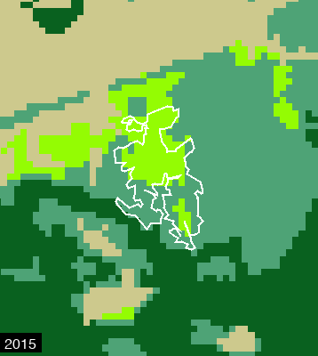

# Export as timestrip (PNG)
export_layer_timestrip(
    site=site,
    layer=MAPBIOMAS_DEFREG,
    output_path='../outputs/defreg_timestrip.png',
    years=[2010, 2012, 2014, 2016, 2018, 2020],
    buffer_m=500,
    tile_size=200
)

# Export as animated GIF
export_layer_gif(
    site=site,
    layer=MAPBIOMAS_DEFREG,
    output_path='../outputs/defreg_timelapse.gif',
    years=range(2010, 2021),
    buffer_m=500,
    dimensions=300,
    duration_ms=600
)

from IPython.display import Image as IPImage
IPImage('../outputs/defreg_timestrip.png')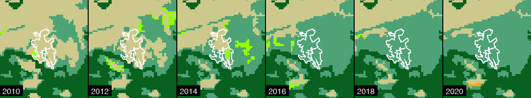

Using generic render_image with any ee.Image

For custom imagery or datasets not wrapped in Layer objects:

site = sites[0]

# Example: Render elevation data
elevation = ee.Image('USGS/SRTMGL1_003')

img = render_image(
    image=elevation,
    region=site.geometry.buffer(2000).bounds(),
    vis_params={'min': 0, 'max': 500, 'palette': ['#0d0887', '#7e03a8', '#cc4778', '#f89540', '#f0f921']},
    dimensions=400,
    boundary=site.geometry,
    label='Elevation (m)'
)
img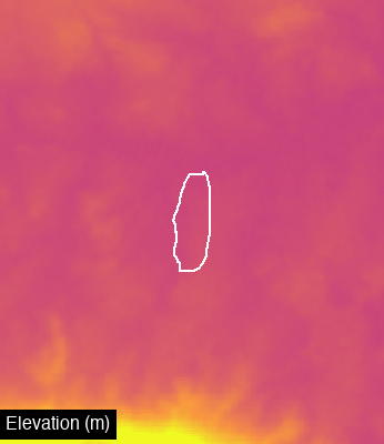

# Example: Sentinel-2 using the dataset helper
from gee_polygons.datasets.sentinel2 import get_sentinel_composite, SENTINEL_VIS

s2_image = get_sentinel_composite(
    geometry=site.geometry,
    date_range=('2020-06-01', '2020-08-31')
)

img = render_image(
    image=s2_image,
    region=site.geometry.buffer(500).bounds(),
    vis_params=SENTINEL_VIS,
    dimensions=400,
    boundary=site.geometry,
    label='Sentinel-2 2020'
)
img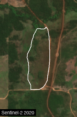

Sentinel-2 Timestrip (2018-2024)

Create a side-by-side comparison of dry season Sentinel-2 composites across multiple years.

# Sentinel-2 timestrip: dry season composites 2018-2024
from gee_polygons.datasets.sentinel2 import get_sentinel_composite, SENTINEL_VIS

frames = []
for year in range(2018, 2025):
    # Get dry season composite (June-August)
    s2_image = get_sentinel_composite(
        geometry=site.geometry,
        date_range=(f'{year}-06-01', f'{year}-08-31'),
        cloud_pct=20
    )
    
    # Render to PIL Image with label
    frame = render_image(
        image=s2_image,
        region=site.geometry.buffer(500).bounds(),
        vis_params=SENTINEL_VIS,
        dimensions=200,
        boundary=site.geometry,
        label=str(year)
    )
    frames.append(frame)

# Export as horizontal strip
export_frames_as_strip(frames, '../outputs/sentinel_2018_2024.png')

from IPython.display import Image as IPImage
IPImage('../outputs/sentinel_2018_2024.png')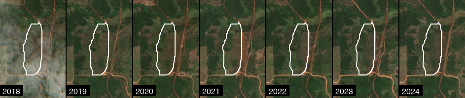

# Also export as animated GIF
export_frames_as_gif(frames, '../outputs/sentinel_2018_2024.gif', duration_ms=700)

Path('../outputs/sentinel_2018_2024.gif')